Package development moved to github

This page is outdated. Please refer to github.com/bgctw/logitnorm.

logitnorm

Utilities for the logitnormal distribution in R

Density, distribution, quantile and random generation function.
Estimation of the mode and the first two moments.
Estimation of distribution parameters.

Download/Install

from download page on R-Forge
To install this package directly within R type: install.packages("logitnorm", repos="http://R-Forge.R-project.org")

Documentaion

The package comes with documentaion and examples. Within R type:

> library(logitnorm)

> `?`(logitnorm)

Distribution

The logitnormal distribution is useful as a prior density for variables that are bounded between 0 and 1, such as proportions. Fig. 1 displays its density for various combinations of parameters mu and sigma.

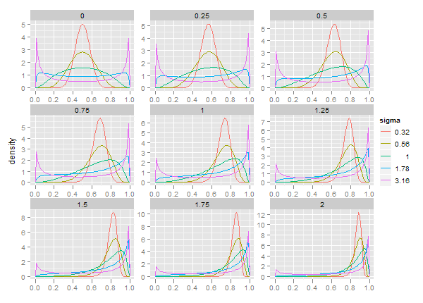
Fig. 1 Density for for various combinations of mu and sigma.

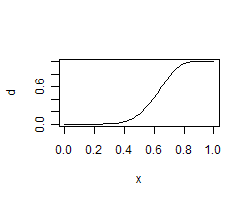
Example: Plot the cumulative distribution

> x <- seq(0, 1, length.out = 81)

> d <- plogitnorm(x, mu = 0.5, sigma = 0.5)

> plot(d ~ x, type = "l")

Mean and Variance

The moments have no analytical solution. This package estimates them by numerical integration:

Example: estimate mean and standard deviation.

> (theta <- momentsLogitnorm(mu = 0.6, sigma = 0.5))

	mean	var
	0.638	0.012

Mode

The mode is found by setting derivatives to zero and optimizing the resulting equation:
$logit(x) = \sigma^2(2x-1)+\mu$

Example: estimate the mode

> (mle <- modeLogitnorm(mu = 0.6, sigma = 0.5))

0.664141601528398

Parameter Estimation

from upper quantile and

mode (Maximum Likelihood Estimate)
mean (Expected value)
median

Example: estimate the parameters, with mode 0.7 and upper quantile 0.9

> (theta <- twCoefLogitnormMLE(0.7, 0.9))

mu	sigma
0.76	0.46

References

Frederic, P. & Lad, F. (2008) Two Moments of the Logitnormal Distribution. Communications in Statistics-Simulation and Computation, 37, 1263-1269

Generated by sweave on: 2010-09-17.

The project summary page you can find here.